Project Ogre Part 2: Building the Digital Twin in Isaac Sim

Creating an accurate digital twin of the mecanum drive robot in NVIDIA Isaac Sim for simulation-first development and testing.

Building the Digital Twin

This is Part 2 of the Project Ogre series. In Part 1, we built the physical mecanum drive robot. Now we'll create an accurate digital twin in NVIDIA Isaac Sim that lets us develop and test without touching the real hardware.

Project Goal: Build an accurate simulation of Project Ogre in Isaac Sim that uses the same ROS2 interface as the real robot, enabling simulation-first development.

📦 Full Source Code: The USD robot model and Isaac Sim configuration are available at github.com/protomota/ogre-slam

Why Simulation First?

In an ideal workflow, you'd build the simulation before touching hardware. I was too eager to get a working robot, so I built the physical platform first. I made progress on the real robot, but eventually hit enough issues that I realized constructing a digital twin would make debugging much easier.

The benefits of simulation-first development:

• No hardware damage risk - Test aggressive maneuvers without breaking motors or sensors

• Faster iteration - Reset the simulation in milliseconds vs. repositioning a physical robot

• Reproducible experiments - Same initial conditions every time

• Parallel development - Work on navigation code while the hardware is being built

Isaac Sim is NVIDIA's robotics simulation platform built on Omniverse. It provides:

• GPU-accelerated physics (PhysX 5)

• Photorealistic rendering with ray tracing

• Native ROS2 integration

• Sensor simulation (LIDAR, cameras, IMU)

The USD Robot Model

The robot is defined in a Universal Scene Description (USD) file: usds/ogre_robot.usd. This format captures geometry, physics properties, and joint definitions in a single file.

Creating the Model

I built the USD model by:

1. Importing the chassis - A simple box representing the steel frame

2. Adding wheel assemblies - Four mecanum wheels with proper roller geometry

3. Defining joints - Revolute joints connecting each wheel to the chassis

4. Setting up collision meshes - Simplified geometry for physics calculations

5. Adding sensors - LIDAR and camera mounts

Physical Dimensions

The USD model matches the real robot's measurements exactly:

Body: 200mm (L) x 160mm (W) x 175mm (H)
Wheel Radius: 40mm
Wheelbase: 95mm (front-to-rear axle distance)
Track Width: 205mm (left-to-right wheel centers)

Getting these dimensions right is critical - SLAM and navigation algorithms depend on accurate odometry, which depends on knowing exactly how far the wheels travel per rotation.

Wheel Configuration

Mecanum wheels require careful attention to roller angles:

M4 (FL) --- M1 (FR)
   |    X    |
M3 (RL) --- M2 (RR)

• Front-left and rear-right wheels have rollers angled one way

• Front-right and rear-left wheels have rollers angled the opposite way

This arrangement creates the characteristic X-pattern when viewed from above. If the roller angles are wrong, the robot won't strafe properly.

Joint Configuration

Each wheel joint needs proper physics parameters for stable simulation:

Joint Properties

# Wheel joint configuration
joint_type: "revolute"
axis: [1, 0, 0]  # Rotate around X-axis
damping: 10.0
friction: 0.1

Critical: Maximum Joint Velocity

Isaac Sim's default maximum joint velocity is extremely high (1,000,000 rad/s). This causes mecanum wheels to spin out of control during physics steps.

Solution: Set maximum velocity to 10,000 rad/s or lower:

drive:
  maxVelocity: 10000.0  # NOT the default 1000000!

This single parameter took hours to debug. The robot would work fine at low speeds but become unstable at higher velocities.

Wheel Sign Correction

The USD model has the right wheels (FR, RR) with opposite joint axis orientation from the left wheels. Sending [+10, +10, +10, +10] to all wheels makes the robot spin instead of moving forward.

The solution is sign correction in the action graph:

Left wheels (FL, RL): velocity as-is
Right wheels (FR, RR): velocity × -1

This normalization ensures [+,+,+,+] always means "all wheels forward" regardless of joint axis conventions.

Physics Settings

Stable mecanum simulation requires tuned physics parameters:

Simulation Timestep

physics_dt: 1/120  # 120 Hz physics
rendering_dt: 1/60  # 60 Hz rendering

The physics timestep must be faster than your control rate. With 30 Hz control, 120 Hz physics gives four physics steps per control step.

Wheel Friction

Mecanum wheel friction is counterintuitive. The angled rollers mean friction behaves differently along different axes:

# Ground material
static_friction: 0.8
dynamic_friction: 0.6

# Wheel material
static_friction: 0.5
dynamic_friction: 0.4

Too much friction and the wheels won't slide sideways. Too little and the robot drifts uncontrollably.

Joint Damping

damping: 1.0 to 10.0  # Range for stability

Damping prevents joint oscillation. Higher values make the wheels feel "heavier" but more stable. Start with 10.0 and reduce if response feels sluggish.

ROS2 Integration

Isaac Sim connects to ROS2 through Action Graphs - visual programming nodes that define data flow.

Setting Up the ROS2 Context

Every Isaac Sim scene with ROS2 needs a context node:

1. Create an Action Graph

2. Add "ROS2 Context" node

3. Set domain_id to match your terminals (default: 0)

The domain ID must match between Isaac Sim and your ROS2 terminals, or topics won't be visible.

Publishing Joint States

To publish wheel positions and velocities:

1. Add "Articulation State" node pointing to the robot

2. Connect to "ROS2 Publish Joint State" node

3. Set topic name: /joint_states

Subscribing to Commands

To receive wheel velocity commands:

1. Add "ROS2 Subscribe Joint State" node

2. Set topic: /joint_command

3. Connect to "Articulation Controller" node

4. Set control type: "velocity"

The Three Action Graphs

Rather than cramming everything into one monolithic action graph, I split the ROS2 integration into three focused graphs. Each handles a specific subsystem, making debugging easier and keeping the visual programming manageable.

Mecanum Drive Controller

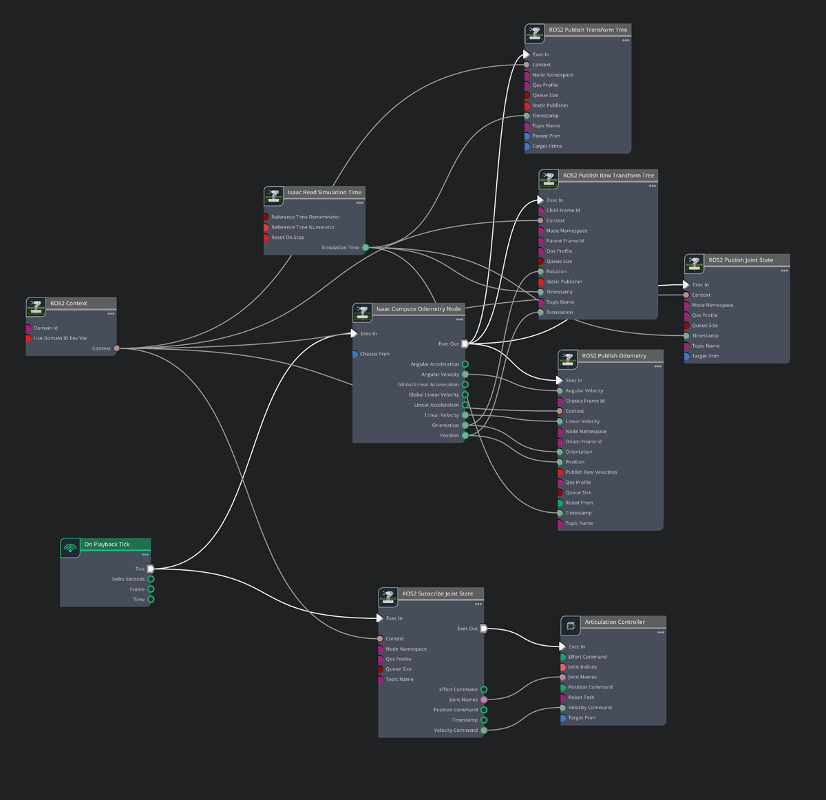
This is the core locomotion graph that handles bidirectional communication between ROS2 and the robot's wheels.

What it does:

• Subscribes to /joint_command for wheel velocity targets

• Applies wheel sign correction (FR, RR × -1) to normalize joint axis conventions

• Drives the Articulation Controller with velocity commands

• Publishes current joint states to /joint_states for odometry feedback

Key nodes:

• ROS2 Context - Establishes the ROS2 bridge with matching domain ID

• ROS2 Subscribe Joint State - Receives velocity commands from the policy controller

• Articulation Controller - Applies velocities to the simulated joints

• Articulation State - Reads current joint positions and velocities

• ROS2 Publish Joint State - Broadcasts state for external nodes

The sign correction happens between the subscriber and the articulation controller. Without it, sending identical velocities to all wheels makes the robot spin instead of driving straight.

LIDAR Sensor Stream

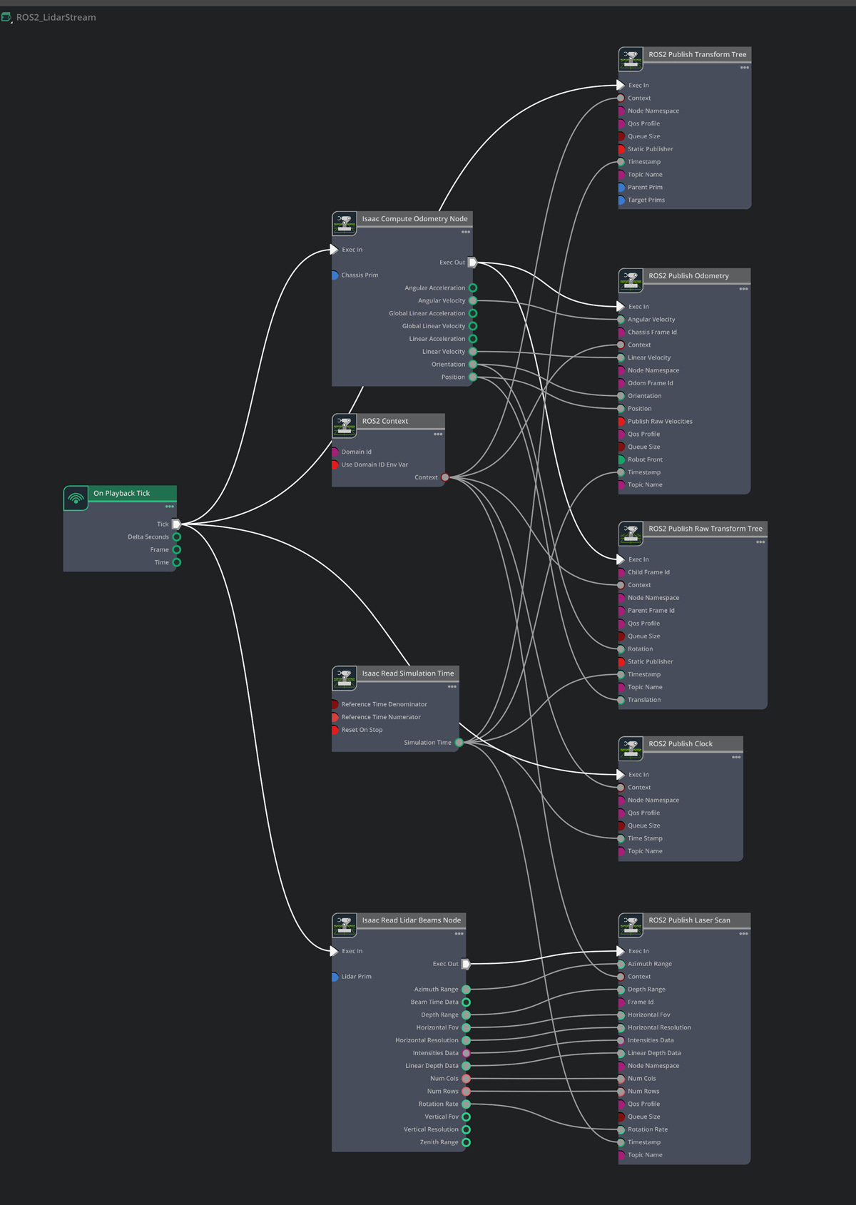
This graph handles the simulated RPLIDAR A1 sensor, streaming 2D laser scan data to SLAM and navigation nodes.

What it does:

• Reads from the RTX Lidar sensor attached to the robot

• Converts the point cloud to a 2D LaserScan message

• Publishes to /scan at the configured rate (~8 Hz to match the real A1)

Key nodes:

• Isaac Read Lidar Point Cloud - Pulls data from the RTX Lidar sensor

• Isaac Create Render Product - Sets up the rendering pipeline for the sensor

• ROS2 Publish LaserScan - Outputs sensor_msgs/LaserScan to /scan

Configuration:

horizontal_fov: 360.0      # Full rotation
horizontal_resolution: 1.0  # 1 degree per sample
max_range: 12.0            # Matches RPLIDAR A1 spec
min_range: 0.15            # Minimum detection distance

The simulated LIDAR matches the real sensor's characteristics closely enough that slam_toolbox configuration works identically in both environments.

RealSense Depth Camera

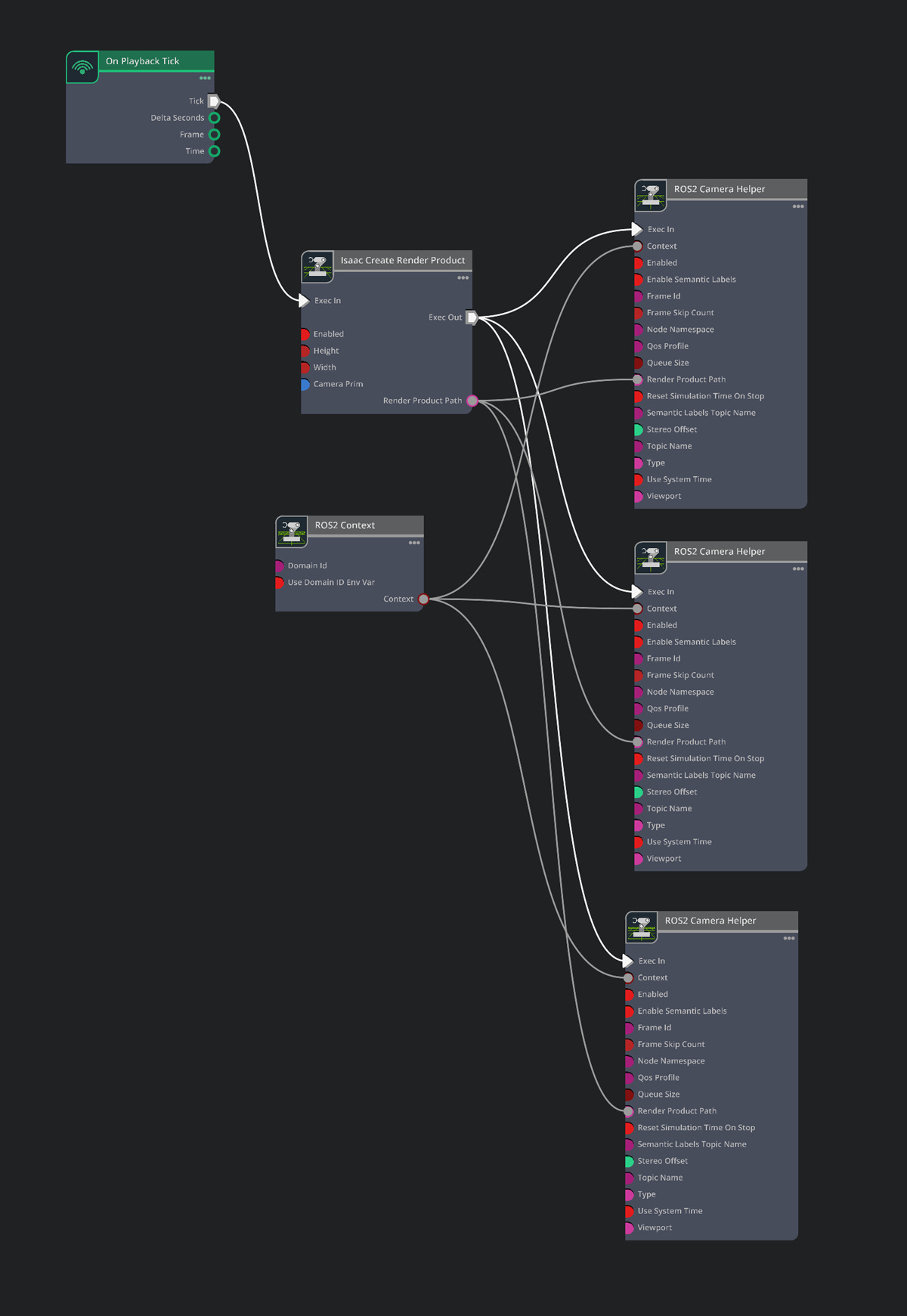
This graph simulates the Intel RealSense D435 depth camera, providing both RGB and depth streams.

What it does:

• Captures RGB frames from the simulated camera

• Generates depth images from the camera's depth sensor

• Publishes synchronized image streams to standard RealSense topics

Published topics:

• /camera/color/image_raw - RGB image (sensor_msgs/Image)

• /camera/depth/image_rect_raw - Depth image (sensor_msgs/Image)

• /camera/camera_info - Camera intrinsics for 3D reconstruction

Key nodes:

• Isaac Create Render Product - Sets up the camera rendering pipeline

• ROS2 Camera Helper - Handles image encoding and publishing

• Isaac Read Camera Info - Extracts camera parameters

Configuration:

resolution: [640, 480]
frame_rate: 30
depth_range: [0.2, 10.0]  # Matches D435 spec

The depth stream feeds into Nav2's voxel layer for 3D obstacle detection - critical for spotting obstacles below the LIDAR's scan plane like table legs or stairs.

Why Three Separate Graphs?

Splitting into three graphs provides several advantages:

1. Isolation - A bug in the camera graph doesn't affect locomotion

2. Performance - Each graph can run at its optimal rate (wheels at 50Hz, LIDAR at 8Hz, camera at 30Hz)

3. Debugging - Easy to disable one sensor while testing another

4. Reusability - The mecanum drive graph works for any 4-wheeled robot

You could combine them into one graph, but the visual complexity becomes overwhelming quickly. Three focused graphs are much easier to maintain.

Testing the Digital Twin

Once the model is configured, test it incrementally:

Step 1: Basic Motion

# Terminal 1: Launch Isaac Sim, load ogre.usd, press Play

# Terminal 2: Send a velocity command
ros2 topic pub /joint_command sensor_msgs/msg/JointState \
  "{velocity: [1.0, 1.0, 1.0, 1.0]}" -r 10

All wheels should spin. If the robot spins in place instead of moving forward, check the wheel sign correction.

Step 2: Omnidirectional Motion

# Forward
ros2 topic pub /cmd_vel geometry_msgs/msg/Twist \
  "{linear: {x: 0.3}}" -r 10

# Strafe left
ros2 topic pub /cmd_vel geometry_msgs/msg/Twist \
  "{linear: {y: 0.3}}" -r 10

# Rotate
ros2 topic pub /cmd_vel geometry_msgs/msg/Twist \
  "{angular: {z: 0.5}}" -r 10

Test all motion primitives. The strafe test is the true mecanum validation - if it moves diagonally instead of purely sideways, check the wheel arrangement.

Step 3: Sensor Verification

# Check LIDAR
ros2 topic echo /scan --once

# Visualize in RViz
rviz2 -d ~/ros2_ws/src/ogre-slam/rviz/isaac_sim.rviz

The LIDAR should show walls and obstacles in the simulation environment.

Simulation vs. Real Robot

The key advantage of this setup: the same ROS2 code runs in both environments.

Component       Simulation         Real Robot
--------------  -----------------  --------------
LIDAR topic     /scan              /scan
Odometry        Isaac Sim physics  Encoder-based
Camera          Simulated RGB-D    RealSense D435
Joint commands  /joint_command     /joint_command

The only difference is launch parameters. The same SLAM, navigation, and control code works in both places.

Simulation-Only Flags

# Simulation
ros2 launch ogre_slam mapping.launch.py use_sim_time:=true

# Real robot
ros2 launch ogre_slam mapping.launch.py use_sim_time:=false

The use_sim_time flag tells ROS2 to use Isaac Sim's clock instead of wall clock. Without this, TF transforms time out because simulation time doesn't match real time.

Common Issues

Robot Falls Through Floor

Cause: Collision meshes not enabled or ground plane missing

Solution:

1. Ensure robot has collision enabled on all rigid bodies

2. Add a ground plane with collision

Wheels Spin But Robot Doesn't Move

Cause: Wheel friction too low or joint damping too high

Solution:

1. Increase ground friction

2. Reduce joint damping

3. Check wheel contact with ground

Robot Vibrates or Explodes

Cause: Physics instability from timestep or mass issues

Solution:

1. Reduce physics timestep (increase Hz)

2. Check mass distribution is reasonable

3. Reduce joint stiffness

Topics Not Visible

Cause: ROS_DOMAIN_ID mismatch

Solution:

1. Check Isaac Sim ROS2 Context domain_id

2. Match in terminal: export ROS_DOMAIN_ID=0

---

Quick Reference

Key Files

File                                   Purpose
-------------------------------------  ----------------------------------------
usds/ogre_robot.usd                    Robot model with physics
usds/ogre.usd                          Complete scene with environment
actiongraph_ros2_mecanum_drive_sm      Wheel control and joint state publishing
actiongraph_ros2_lidar_stream_sm       LIDAR sensor simulation
actiongraph_ros2_real_sense_camera_sm  RGB-D camera simulation
rviz/isaac_sim.rviz                    RViz config for simulation visualization

Isaac Sim Settings

Physics:
  timestep: 1/120 (120 Hz)
  solver_iterations: 4

Wheel Joints:
  max_velocity: 10000 rad/s
  damping: 10.0

Ground:
  static_friction: 0.8
  dynamic_friction: 0.6

What's Next

With the digital twin working, Part 3 covers using slam_toolbox to build maps. We'll run SLAM in both simulation and on the real robot, comparing results and tuning parameters for accurate mapping.

The ability to test SLAM in simulation before deploying to hardware saves significant time - you can iterate on configuration without draining the robot's battery or worrying about collisions.